


Next: Representation
Up: Completely bounded bilinear mappings
Previous: Jointly complete boundedness
Contents
Index
Complete boundedness
For the definition of the
completely
bounded
bilinear maps we need
the
amplification
 ,
the linearization
,
the linearization
 .
and the
tensor matrix multiplication
.
and the
tensor matrix multiplication
 of operator matrices
  ,
,  .
A bilinear mapping
.
A bilinear mapping
 ,
,
 is called completely bounded if
where
,
is called completely bounded if
where
,
 ,
,
 .
The norm
.
The norm
 equals the norm
 of the linearization
on the Haagerup tensor product.
Furthermore,
the norms
of the linearization
on the Haagerup tensor product.
Furthermore,
the norms
 are obtained using the
tensor matrix products
of all 49 rectangular matrices of
are obtained using the
tensor matrix products
of all 49 rectangular matrices of  rows resp. columns:
where
rows resp. columns:
where
 ,
,
 ,
,
 .
We have
The norm
equals the norm
.
We have
The norm
equals the norm
 of the amplification of the linearization
on the Haagerup tensor product.
A bilinear form
of the amplification of the linearization
on the Haagerup tensor product.
A bilinear form  is already seen to be completely bounded if
 .
Then we have
.
Then we have
 .50
.50
 denotes the operator space consisting of completely
bounded bilinear maps.
One obtains a norm on each matrix level using the identification
Corresponding to the completely bounded bilinear maps we have the
linear maps which are completely bounded on the
Haagerup tensor product .
The identification
holds completely isometrically.
Completely bounded bilinear mappings are in particular
jointly completely bounded.
The embedding
denotes the operator space consisting of completely
bounded bilinear maps.
One obtains a norm on each matrix level using the identification
Corresponding to the completely bounded bilinear maps we have the
linear maps which are completely bounded on the
Haagerup tensor product .
The identification
holds completely isometrically.
Completely bounded bilinear mappings are in particular
jointly completely bounded.
The embedding
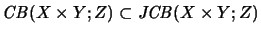 is a complete contraction.
The transpose
is a complete contraction.
The transpose
 of a completely bounded
bilinear mapping in general is not completely
bounded.51
For completely bounded bilinear
(and, more generally, multilinear) maps
of a completely bounded
bilinear mapping in general is not completely
bounded.51
For completely bounded bilinear
(and, more generally, multilinear) maps
 we have some
generalizations
of Stinespring's representation theorem.
we have some
generalizations
of Stinespring's representation theorem.
Footnotes
- ... all49
- Note that the norm of the bilinear map
in general is smaller than the norm
.
- ....50
- More generally, the equation
holds for bilinear maps with values in a commutative C
 -algebra
  since every bounded linear map taking values in
is automatically completely bounded and
since every bounded linear map taking values in
is automatically completely bounded and
 [Loe75, Lemma 1].
For bilinear maps
[Loe75, Lemma 1].
For bilinear maps
 we have
 .
.
- ...51
- To this corresponds the fact that the
Haagerup tensor product
is not symmetric.
Next: Representation
Up: Completely bounded bilinear mappings
Previous: Jointly complete boundedness
Contents
Index
Prof. Gerd Wittstock
2001-01-07